Factoring With Geometry: Lestra’s Method

An introduction to a fascinating integer factorization algorithm, told in five parts.

This article is a reformatted version of my submission to the Summer of Math Exposition 2 (SoME2) contest hosted by the YouTube creator 3Blue1Brown. You can find the original article here.

In this article, I want to tell you about one of my favorite mathematical algorithms: Lenstra’s method. It is an algorithm for factoring large integers which approaches the problem from a unique perspective. In order to understand how this algorithm works, I’ll need to take you on a journey through the world of number theory.

(DISCLAIMER) I’ve written this article to be approachable to students from all different levels of math. As a result, the proofs below are not especially rigorous, though I strive to maintain depth and accuracy with my explanations. My goal is to build intuition and enthusiasm, but if you would like a more comprehensive, formal, and rigorous description of Lenstra’s method, I encourage you to consult the resources located at the bottom of this article.

Part 1 — In Search of a Factor

Integer factorization holds an essential role in mathematics. Breaking apart a number into its component primes finds a wide array of uses across the various, seemingly disjunct, domains of mathematics. To name a few examples, in algebra, integer factorization helps mathematicians determine the possible decompositions of a finite abelian group. In number theory, crucial important theorems such as the Chinese Remainder Theorem and Euler’s Theorem depend upon knowing how a given number factors. The list of applications of factorization could go on and on. Factorization is one of the most powerful techniques in the mathematician’s toolkit, yet despite its profound importance, I would wager that the factorization method you were taught is highly inefficient. Why is this?

Say we want to factor 5040. Here’s how you would probably go about it. We know that the first five prime numbers are 2, 3, 5, 7, and 11, so why don’t we try to divide 5040 by each of these numbers? 2 divides four times, 3 divides twice, 5 divides once, seven divides once, and eleven does not divide at all. Luckily for us, these happen to be the only prime factors of 5040.

$$\large{\displaystyle 5040 = 2^4 \cdot 3^2 \cdot 5 \cdot 7}$$

The prime factorization for 5040.

This approach is known as the trial division algorithm. It is the simplest and most straightforward of the factorization algorithms. It is the method every student is first taught and, for many, it is the last they will ever learn. But there is so much more to factoring. Perhaps understanding what is wrong with the trial division algorithm serves as a good place to start on our journey.

The trial division method is all well and good provided that we can do two things. First, we must be able to efficiently generate a list of prime numbers. Both the Sieve of Eratosthenes and Sieve of Atkin permit us this possibility so this first requirement is not a huge concern. That is, assuming that the number we are factoring has prime factors within our repository of primes. This caveat brings us to the second condition, which poses more of an issue. The trial division algorithm only works efficiently provided that we know that the prime factors of the number are small.

Consider a very large number such as 6,755,386,553,008,134 (6 quadrillion, 755 trillion, 386 billion, 553 million, 8 thousand, and 134 — quite the mouthful, isn’t it?). It can be verified that this number is divisible by 2 and 3, but its only other prime factors are relatively large — 524,287 and 2,147,483,647. We would have to iterate through our list of primes for quite a while until we “hit” these factors. This number could be factored by trial division by a computer after some time, especially since the first large prime (524,287) appears much earlier than the second (2,147,483,647), but it would be easy to conceive of a number so large that trial division would not halt after a reasonable period of time. With trial division, we would be unnecessarily checking the divisibility of our number by a bunch of “misses” as opposed to the sparser “hits” —the numbers we actually care about. Checking divisibility like this is an incredibly wasteful process and, for numbers with exceptionally large prime factors, the trial division algorithm would take ages before it finishes.

$$\large{\displaystyle 6\,755\,386\,553\,008\,134 = 2 \cdot 3 \cdot 524\,287 \cdot 2\,147\,483\,647}$$

The prime factorization for the monstrously large number 6,755,386,553,008,134. Well… by a mathematician’s standard, this number is relatively small. It’s got nothing on the size of the monster group!

Managing this “hit/miss” ratio is why prime factorization is such a hard problem to solve. In fact, the search for a quick factorization algorithm remains an unsolved problem in computer science. As well, the security of RSA public-key cryptography depends upon this inability to factor large numbers within a reasonable amount of time. This is a win for privacy, but a devastating loss for us pure mathematicians.

Trial division thus leaves us with a problem. How can we increase our hit rate?

Part 2 — In Search of a Solution

In 1974, a British mathematician named John Pollard published a factoring algorithm known as $p-1$. The power of this method comes from how it substantially reduces the total number of “misses” we consider. Proving this method relies on some algebra that may seem counterintuitive at first or like some sort of mathematical trickery — at least, it seemed that way to me at first. It is my hope that, by the end of the proof, it will be clear that every step was done for an important reason.

The proof of $p-1$ is done by means of a theorem known as Fermat’s Little Theorem, not to be confused with its older and more infamous brother: Fermat’s Last Theorem.

Fermat’s Little Theorem states that for any prime $p$ and any positive integer $\alpha$, if $\alpha$ raised to the power of $p$ is divided by $p$, then the remainder equals the remainder of $\alpha$ divided by $p$.

For instance, if $\alpha = 12$ and $p = 7$, we know that $12^7 = 35,831,808$ divided by 7 leaves a remainder of 5 since $12/7$ leaves a remainder of 5.

$$\large{\displaystyle \alpha^p \equiv \alpha \pmod{p}}$$

Fermat’s Little Theorem. For those unfamiliar with the notation, the (mod p) denotes that we should divide both sides of the equation by p and return the remainder. Note that, whenever we invoke the “mod” operation, we call the divisor the modulus. In addition, that “triple equals” sign simply means that the two numbers share the same remainder after division by p.

Now consider what happens if we divide both sides by $\alpha$ and raise both sides of this equation by some positive integer $m$.

$$ \large{\displaystyle \alpha^{p-1} \equiv 1 \pmod{p}} \\ \large{\displaystyle \alpha^{m(p-1)} \equiv 1^m \pmod{p}} \\ \large{\displaystyle \alpha^{m(p-1)} \equiv 1 \pmod{p}} $$

In the first step, we divide both sides by alpha. It should be noted that I can’t always divide both sides of a modular equation by a common factor. But, because of reasons that will be apparent later, this step is in fact justifiable because alpha and p are coprime; hence the modular inverse of alpha exists. In the second and third steps, we raise both sides of the equation to the power of an arbitrary integer m.

Finally, if we subtract one from both sides, we arrive at an equation that expresses divisibility — precisely the type of equation we are looking for.

$$\large{\displaystyle \alpha^{m(p-1)} - 1 \equiv 0 \pmod{p}}$$

The result of subtracting 1 from both sides of the modular equation. This result tells us that p must evenly divide the expression on the left since the division results in a remainder of zero.

So we know that $p$ divides that expression on the left. So what? How does this relate to factoring any arbitrary integer? Well, suppose we want to find a factor of the number $n$. We know that all integers greater than one have at least one prime factor. And we just proved, by Fermat’s Little Theorem, that whatever prime factor $n$ is divisible by will also evenly divide into that weird $\alpha$ expression. Since $n$ and that $\alpha$ expression share the common factor $p$, then their greatest common divisor cannot equal one. And, by the definition of the greatest common divisor, the gcd will be the factor of $n$ that we are looking for.

$$ \large{\displaystyle \text{Let } n \text{ be an arbitrary natural number such that } p \text{ divides } n} \\ \large{\displaystyle p \text{ also divides } \alpha^{m(p - 1)} - 1} \\ \large{\displaystyle n \text{ and } \alpha^{m(p - 1)} - 1 \text{ must share a common factor}} \\ \large{\displaystyle \text{Therefore } \gcd(n, \alpha^{m(p - 1)} - 1) \neq 1} $$

A restatement of the above logic. p is a prime factor of both n and the alpha expression.

But wait! We’ve hit a snag in our analysis. In order to find a factor of $n$, we need to know what $p-1$ is. But if we knew a prime $p$ that divides into $n$, then we wouldn’t need all this math in the first place! Luckily for us, we don’t actually need to know $p$.

What if we assumed that $p-1$ is composed of a small number of small prime factors? As an example, if $p = 524,287$, then $p-1$ is equal to a product of a small number of small primes ($p-1 = 524286 = 2 \cdot 3^3 \cdot 7 \cdot 19 \cdot 73$). By the way, what counts as “small” is mostly up to personal interpretation and is ultimately determined by how long we want our algorithm to take to find a factor.

If this assumption happens to hold true for a prime number $p$ that divides our $n$, then we might be able to find some number $k$ that happens to contain all of the factors that $p-1$ has. In other words, $k$ will take the place of $m(p-1)$.

$$ \large{\text{Let } k = m(p - 1)} \\ \large{\text{Then } \displaystyle \alpha^{k} - 1 \equiv 0 \pmod{p}} \\ \large{\text{We assume } p-1 \text{ factors as } q_1^{\beta_1}q_2^{\beta_2}...q_N^{\beta_N}} \\ \large{\text{ where } q_i, \beta_i, \text{ and } N \text{ are "small"}} $$

A restatement of the "small prime factors" assumption.

What should this $k$ be? There are all sorts of numbers we could try, but let’s use the least common multiple to generate $k$, since this will allow us to quickly generate large numbers containing a small number of small prime factors. You can use whatever procedure you want, so long as the resulting number has a lot of prime factors.

Consider the least common multiple of the first ten positive integers. This number would be divisible by a small number of twos, a small number of threes, some fives, and some sevens.

$$ \large{\text{lcm}(1,2,3,4,5,6,7,8,9,10) = 2520} \\ \large{2520 = 2^3\cdot 3^2\cdot 5\cdot 7} $$

An example of a possible k we may choose.

We can think of this least common multiple as a blob of mushed-together factors. The more integers we consider - 100, 1000, 10000 (although in practice significantly larger numbers such as $10^10=10,000,000,000$ are used) - the larger this blob becomes and, more importantly, the higher the likelihood that it will contain all of the factors of $p-1$, whatever $p$ may be.

We are essentially playing a guessing game: we choose an arbitrary number of positive integers, find their least common multiple, and hope that $p-1$ will divide it. This process relies on a bit of luck, but it does not require us to know anything about $n$’s factors.

With Pollard’s method we now have a new method for generating “hits”. Here’s the full algorithm:

Select a number $n$ that you want to factor. Then choose any number $\alpha$ that doesn’t share a factor with $n$ ($\alpha$ would then be said to be coprime with $n$). We could use $\alpha = 2$, for instance, since $n$ will be guaranteed to be odd (if $n$ was even, we could continually divide $n$ by 2 until we are left with something indivisible by 2).
$$\large{\text{Step 1: Choose } \alpha \text{ coprime with } n}$$
We then set a value of $B$, known as our smoothness bound, which limits the largest prime factor $k$ will be divisible by. Next, we let $k$ be the least common multiple of the first $B$ positive integers. We then compute $d$, our potential factor.
$$ \large{\text{Step 2a: Choose } B} \\ \large{\text{Step 2b: Let } k = \text{lcm}(1, 2, ..., B)} \\ \large{\text{Step 2c: Let } d = \gcd(n, \alpha^k - 1)} $$
If $d$ is neither 1 nor $n$ (a.k.a: the “trivial” factors), then we have found a valid factor of $n$, meaning our choice of k was a “hit” and we can halt the algorithm. If not, and $d$ is 1 or n, then our $k$ value was a “miss” and we must either select a new value for $B$ or, if that doesn’t work, we must instead select a different $/alpha$ and try again.
$$ \large{\text{Step 3: } \begin{cases} \text{Factor Found!} & d \neq 1 \text{ and } d \neq n\\ \text{Try again!} & d = 1 \text{ or } d = n \end{cases} } $$

Note that Pollard’s method doesn’t factor $n$ completely, nor does it guarantee that the resulting factor is prime. All it does is find a single factor of $n$. To find $n$’s prime factorization, we run Pollard’s method to get some factor of $n$, find the prime factorization of this factor - usually with a simpler method like trial division if the factor is small - and we divide $n$ by Pollard’s factor repeatedly until $n$ can no longer be divided evenly. To confirm that a given factor is prime, one could use a primality checking algorithm such as the Miller-Rabin primality test. We then repeat the process over again, making $n$ smaller and smaller, until no more factors can be found. We will then have completely factored $n$ into its component prime factors.

Though a little strange, Pollard’s $p-1$ algorithm greatly improves upon the “hit/miss” detection that we saw with trial division. But, the method is not without its flaws. If $p-1$ is not a product of small primes, like we assumed, we would be in considerable trouble. We would be forced to resort to an unreasonably large smoothness bound and there would be no hope of the algorithm halting within a reasonable amount of time.

Perhaps we could yet again improve our “hit/miss” detection and further expand upon what makes Pollard’s method so powerful.

And in 1987, a Dutch mathematician named Hendrik Lenstra did just that. But he approached the problem of factoring from a new perspective. What if we stopped thinking about numbers… and started thinking about curves? Bear with me.

Hendrik Lenstra

Hendrik Lenstra, who teaches at the Leiden University in the Netherlands.

Part 3 - A New Perspective

Lenstra’s method relies on a class of curves known as elliptic curves. Elliptic curves have long been studied in one form or another by mathematicians since the days of Fermat in the 17th century, and they find a wide range of applications across number theory. For instance, elliptic curves were instrumental in Andrew Wiles’s proof of Fermat’s Last Theorem (that pesky Fermat keeps rearing his head!). Despite the apparent simplicity of the elliptic curve equation, there is immense complexity hidden within.

Pierre de Fermat

You cannot escape Fermat. He will follow you into all of your mathematical endeavors…

And before you ask, no. Elliptic curves are not ellipses. Elliptic curves are not all that related to ellipses either - at least, based on how I will be presenting them in this article. But there is a reason for this nomenclature - it is just beyond the scope of this article. In short, the term “elliptic” refers to the elliptic integrals used to compute the arc lengths of ellipses.

An elliptic curve is an equation of the form $y^2= x^3 + ax + b$ (which I will occasionally denote by $E_{a,b}$). The curve is symmetric about the x-axis and bulges at its center.

Elliptic Curve Example

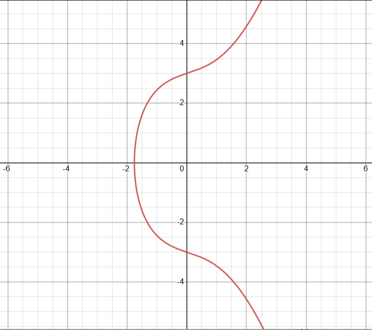
A graph of the elliptic curve y² = x³ + 2x + 9.

One neat property of these curves is that, depending on our choice for $a$ and $b$, an elliptic curve can be divided two components: one “mainland” curve and an “island” curve.

Elliptic Curve Division

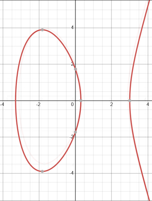
A graph of the elliptic curve y² = x³ - 10x + 3. This time, the elliptic curve consists of two distinct components: the "mainland" curve (right) and the "island" curve (left).

When we use elliptic curves in number theory, we often want to compute points on an elliptic curve with respect to some modulus. For instance, we might want to find the set of all integer points $(x, y)$ on some elliptic curve mod 10. It should be noted that, when we do this, we are only considering rational solutions to our modular elliptic curve. By taking the modulo of our elliptic curve, we don’t get a continuous curve like before, but instead, we get a seemingly random scattering of points. What’s more, our elliptic curve is much smaller. Whereas before we had infinitely many real points on the curve, we now have finitely many integer points. As counter-intuitive as it seems, this scatterplot is still our elliptic curve, just from the perspective of each point’s remainders. Evaluating elliptic curves in this peculiar way grants us some very important properties for factoring numbers, as you will soon see.

An animation of the process of transforming an elliptic curve into its modular twin (or more accurately a subset of points on its modular twin). Don't worry if the animation looks a little "hand-wavy" - it's a weird transformation. What's happening is that we identify all of the points on the original elliptic curve that are rational - whose coordinates are capable of being written as a ratio of integers. We can then map these rational points to integer points in the modular plane using a process that will be described later on in the article.

Remember that, for any elliptic curve, we can construct a corresponding modular elliptic curve. We won’t be using this technique just quite yet, but it will serve us well later on.

What does it mean to add? This may seem like an odd tangent considering I was just talking about curves, but creating a relatively formal definition for addition will aid us with factoring.

Well, our definition of addition is entirely dependent on what it is that we wish to add. Adding integers is different from adding complex numbers which is different from modular addition. These are relatively simple examples, but they illustrate the simple principle that even commonplace operators have different behaviors depending on the set of “things” that they act upon.

Suppose we define an operation called addition that takes any two elements in a set and returns another object in the same set. Because our addition operator acts on two elements at once, we call it a binary operation. This operation and its underlying set form a structure mathematicians call a group. I will denote the group for our generalized addition as G. But what features should this group have?

The addition operator should be associative. This means that:

$$\large{(a + b) + c = a + (b + c) \text{ for } a, b, c \in G}$$

The definition of associativity for a group G. Associativity means that we may insert brackets/parentheses however we please into our expressions. It does not mean that we may swap the order of a, b, or c. As a side note, if you are unfamiliar with that backwards-three/epsilon symbol, it means that a, b, and c are elements of the underlying set of G.

There should exist an object, called an identity/normal, that when added to any element in the set leaves it unchanged. This identity, which I’ll denote by $e$, is unique and satisfies the following for all elements in the group:

$$\large{a + e = e + a = a \text{ for } a \in G}$$

The definition of identity for a group G. If our group was the set of integers with the binary operation between integers being addition, then the identity element would be zero. If the binary operation was instead multiplication, then the identity element would be one.

For all elements in the set, there should also exist a unique inverse in our set that, when added to the original element, produces our identity. I will denote the identity of any $a$ in our group by $-a$.

$$\large{a + (-a) = (-a) + a = e \text{ for } a \in G}$$

The definition of inverse for a group G. If our group was the set of integers with the binary operation between integers being addition, then the identity element would be the negation of the element (2's inverse would be -2 since 2 + (-2) = 0). If the binary operation was instead multiplication, then only 1 and -1 would have inverses since all other integers would have non-integer inverses (for instance, 2's inverse would be 1/2 which is not an integer). This means that the set of integers with the addition operator forms a group, but the set of integers with the multiplication operator does not form a group.

The addition operator should be commutative for all $a$ and $b$ in our group. Because of the commutative nature of addition, this distinguishes addition as a special type of group known as an abelian group, named after the Norwegian algebraist Niels Abel.

$$\large{a + b = b + a \text{ for } a, b \in G}$$

The definition of commutativity for a group G. Commutativity means that we may swap the inputs to our binary operator and we would still get the same result. Combined with associativity, this means that any sequence of additions can be ordered and evaluated however we want.

The addition operator should be closed, meaning that if we were to add any two elements a and b in our group, we would be guaranteed a sum that is also in our group. Our group will be completely contained. With closure, we do not need to worry that an element outside of our group will be created, thereby creating undefined behavior if we were to add this external element to any of the elements in our group.

Side note: this may seem like a lot of properties to remember, but these restrictions are just a formalization of the intuition we already have surrounding addition. And, more generally, groups are just a formalization of the notion of symmetry. If you are interested, 3Blue1Brown has a very good video about this connection between group theory and symmetry.

Now, back to elliptic curves.

Suppose we have two points $P$ and $Q$ on an elliptic curve. What would it mean to add these two points? We could try adding the $x$ and $y$ coordinates of each point, but this definition of point addition fails to be closed — we would not be guaranteed a point that lies on our elliptic curve. For instance, $(0,2)$ and $(1,3)$ are points on the elliptic curve $E_{4,4}: y^2 = x^3 + 4x + 4$, but $(1,5)$ is not. Our definition for addition on an elliptic curve instead needs to satisfy the properties of an abelian group.

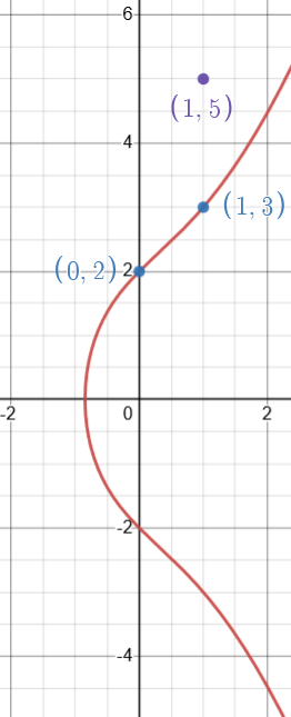
Whoops! This is a failed attempt at adding the points (0, 2) and (1, 3) on the elliptic curve y² = x³ + 4x + 4.

Instead, to compute the sum of $P$ and $Q$, we first draw a line connecting the two points. Because of the shape of elliptic curves, the line connecting $P$ and $Q$ will either intersect the elliptic curve at a point distinct from $P$ and $Q$ or will never intersect the curve at all.

If $P = Q$, then we would be unable to draw a secant line between the two points. We must instead draw a tangent line. Once again, the tangent line will intersect the curve at one other point or not at all. This is how we will double $P$.

We are now left with two cases to consider.

Case 1: The line connecting $P$ and $Q$ intersects the elliptic curve.

The first case is relatively straightforward. Through some algebra, we can precisely compute which point $R$ the line will intersect the curve at. We then reflect this point of intersection across the $x$-axis by negating its $y$-component. We denote this reflection by $-R$. Thus, $P + Q = -R$. If negating the intersection point seems strange, don’t worry. There is a reason for this, though you’ll have to wait for an answer.

$$\large{P + Q = -R}$$

The fundamental equation for point addition on an elliptic curve. Look how simple it is! Well… it's only simple because it's been abstracted. P and Q are points on our elliptic curve, R is our point of intersection between the line PQ and the elliptic curve, and -R is R's reflection about the x-axis.

An animation of point addition on an elliptic curve. The first animation demonstrates how to add two distinct points on an elliptic curve and the second animation demonstrates how to double a point on an elliptic curve.

Case 2: The line connecting P and Q DOES NOT intersect the elliptic curve.

The second case is weirder. If the line never intersects the curve, then we won’t be able to add two points to get a third distinct point on the curve. But if our point addition isn’t closed, how can it be addition at all?

But suppose there is a third point. What would this hypothetical point “on” the curve look like? Well, this point would only show up if $Q$ was a reflection of $P$ about the $x$-axis since the line joining these two points would be vertical. This hypothetical point of intersection with the curve, which I will denote as $O$ (this is an “oh”, not a zero), is what is known as an infinity point/point at infinity which lies at the limits of our vertical line. We then have two possible “points” to choose from: one at $y = \infty$ and another at $y = -\infty$. It turns out that both of these points refer to the same $O$.

An animation showing the addition of two points on an elliptic curve, where each point is the x-axis reflection of the other. This creates the infinity point, which lies at the extremes of the vertical line joining the points.

So we have that $P + (-P)$ equals $O$. The infinity point solves the problem of symmetric points and leads to some other interesting consequences. What would $P + O$ look like? Well, the third point of intersection on the curve would be $-P$ (since the line joining $P and O$ would be vertical) and, after reflecting $-P$, we would get $P$, meaning that $P + O = P$. In fact, the reason we reflect the point of intersection at all is precisely because we want our infinity point to leave $P$ unchanged under addition.

$$ \large{P + (-P) = O} \\ \large{P + O = P} $$

The “infinity point” identities for elliptic curve point addition.

We now have identified two types of special points: for any point $P$, $-P$ would be the inverse element of $P$ and $O$ would be our identity element. Essentially, the infinity point ends up playing a role similar to the role zero plays in the addition of real numbers.

But hold on just a minute. Points at infinity? What’s going on here?! This doesn’t make any sense! Surely mathematicians are pulling our leg here…

Don’t worry if you find the infinity point a little confusing. I think the entire idea of an infinity point is counter-intuitive. Even with all the research I’ve done, I still find it a little unbelievable. Why are mathematicians allowed to make up non-existent points like this and assume they exist “on” the curve? How can a point exist at infinity?

As confusing as it is, I like to think of it as an extension of our notion of a point to help us later on with our calculations. Infinity points are just like imaginary numbers in a way: both appear at first to defy reality and common sense, yet both serve essential purposes and possess rigorous mathematical definitions.

The strangeness of the infinity point appears to follow as a consequence of simplifying elliptic curves to a 2D representation. In reality, elliptic curves are actually a functions of 3 variables: $X, Y, Z$.

$$ \large{y^2 = x^3 + ax + b} \\ \large{\downarrow} \\ \large{Y^2Z = X^3 + aXZ^2 + bZ^3} \\ \large{\text{Where } x = X/Z \text{ and } y = Y/Z} $$

An elliptic curve in 3 variables. We often restrict X, Y, and Z to integers so that solutions (x, y) to the 2D case are rational.

We describe points on this curve in homogeneous coordinates $[X : Y : Z]$. In this system, every $[X : Y : Z]$ maps to the same point in the Cartesian plane as $[kX : kY : kZ]$ for some non-zero real number $k$. Furthermore, we omit the point $[0 : 0 : 0]$ from our coordinate system. Thus, the elliptic curve of three variables above (in homogeneous coordinates) has been projected onto the 2D plane by $x = X/Z$ and $y = Y/Z$; this is why the infinity point doesn’t make sense. $(0, 1, 0)$ and all of its multiples are valid solutions to the elliptic curve in homogeneous coordinates, but they undergo a strange transformation when they are projected onto the Cartesian plane because of a division by zero. Thus, in the 2D case, $(0, 1, 0)$ (and all its multiples) become the “infinity point”. In this sense, the infinity point still maintains its uniqueness since $[0 : 1 : 0]$ and $[0 : 2 : 0]$ are treated as effectively the same point. There will never be multiple infinity points because every point of the form $[0 : k : 0]$ is an infinity point.

In addition, one can also show using homogeneous coordinates that the line connecting any $P$ and its inverse intersects at the infinity point $O$.

I omitted all this initially because I personally find it much easier to visualize 2D elliptic curves despite them being technically incorrect. We will continue to think about elliptic curves on the Cartesian plane, but know that this representation brings with it some unintended quirks and only scratches the surface of the complexity of Elliptic curves.

Though I will not prove all of these properties, our definition of point addition now satisfies the requirements for an abelian group. For any points $P$, $Q$, and $R$ on the elliptic curve, point addition…

Is closed, meaning that adding two points on the curve will produce another point on the curve or will produce our infinity point.
Is associative, meaning that:

$$\large{(P + Q) + R = P + (Q + R) \text{ for } P, Q, R \in E_{a, b}}$$

Associativity of elliptic curve point addition.

Is commutative, meaning that:

$$\large{P + Q = Q + P \text{ for } P, Q \in E_{a, b}}$$

Commutativity of elliptic curve point addition.

Has a “unique” identity element — our infinity point $O$:

$$\large{P + O = O + P = P \text{ for } P \in E_{a, b}}$$

The rules for the identity element of our elliptic curve group.

Admits a unique inverse element $-P$, the reflection of $P$ across the x-axis, for every point:

$$\large{P + (-P) = (-P) + P = O \text{ for } P \in E_{a, b}}$$

The rules for the inverse of any element of our elliptic curve group.

Part 4 - Bringing It All Together

In the last section, we derived the geometric meaning behind adding points on an elliptic curve. But how do we explicitly compute their sum? To do so requires drawing some line, seeing where that line intersects the elliptic curve, and negating the point of intersection.

If the points are distinct, but $Q$ is not a reflection of $P$ (since this would mean that $P + Q = O$), then we draw the secant line between them. To find the intersection point, we make the substitution $y = mx + \beta$ and rearrange the resulting equation.

$$ \large{\text{Define } P = (x_P, y_P) \text{ and } Q = (x_Q, y_Q)} \\ \large{\text{Line } \overline{PQ} \text{ is defined by } y = mx + \beta} \\ \large{\text{Where } m = \frac{y_Q - y_P}{x_Q - x_P} \text{ and } \beta = y_P - mx_P} $$

The parameters of the line PQ joining P and Q and intersecting the elliptic curve at some distinct third point.

$$ \large{(mx + \beta)^2 = x^3 + ax + b} \\ \large{m^2x^2 + 2m\beta x + \beta^2 = x^3 + ax + b} \\ \large{x^3 - m^2x^2 + (a - 2m\beta)x + (b - \beta^2) = 0} $$

Substituting mx + beta into the general elliptic curve equation y² = x³ + ax + b. Note that I subtracted everything on the left from the right and I swapped the left and right hand sides of the equation in the last step.

This gives us a cubic equation with three roots. In fact, we already know what the three roots are going to be since we already know three points on the line $\overline{PQ}$: the first root is P’s x-coordinate, the second root is Q’s x-coordinate, and the third root is the x-coordinate of the point of intersection R.

$$ \large{x^3 - m^2x^2 + (a - 2m\beta)x + (b - \beta^2) = (x - x_P)(x - x_Q)(x - x_R)} \\ \text{Comparing the coefficients gives us} \\ \large{m^2 = x_P + x_Q + x_R} \\ \large{a - 2m\beta = x_Px_Q + x_Qx_R + x_Rx_P} \\ \large{\beta^2 - b = x_Px_Qx_R} $$

Equating the above polynomial with its factored representation allows us to compare the coefficients of each term. Each equation relating the cubic's coefficients with its roots can be determined by expanding the factored representation and comparing like-terms or by simply applying Vieta's Formulas.

If we compare the coefficients between the left and right sides of the equation, we arrive at three equations. But actually, only the first equation is necessary to determine what R’s x-coordinate is.

$$ \large{m^2 = x_P + x_Q + x_R} \\ \large{x_R = m^2 - x_P - x_Q} $$

Using the first relationship between roots and coefficients, we can arrive at a formula for R's x-coordinate.

From here, we can substitute this x into our secant line equation (y = mx + beta) to find R’s corresponding y-component, and we finally negate the y-coordinate to arrive at an explicit formula for the sum of two points on an elliptic curve.

$$ \large{P + Q = (x_R, -mx_R - \beta)} \\ \large{x_R = m^2 - x_P - x_Q} \\ \large{\text{Where } m = \frac{y_Q - y_P}{x_Q - x_P} \text{ and } \beta = y_P - mx_P} $$

The explicit formula for the addition of two distinct points on an elliptic curve under the assumption that Q is not a x-axis reflection of P.

Now what if $P = Q$? In other words, how would we go about doubling $P$?

Well, we must instead draw the tangent line to the elliptic curve at $P$. If we apply the derivative with respect to $x$ on both sides of our elliptic curve equation and solve for $\displaystyle \frac{dy}{dx}$, we can find the slope of the tangent line at any given $x$.

$$ \large{\displaystyle \frac{d}{dx}(y^2) = \frac{d}{dx}(x^3 + ax + b)} \\ \large{\displaystyle 2y\frac{dy}{dx} = 3x^2 + a} \\ \large{\displaystyle \frac{dy}{dx} = \frac{3x^2 + a}{2y}} $$

Deriving the formula for the slope of a line tangent to an elliptic curve. Notice how the derivative is undefined precisely when y = 0 - when the bulge of the elliptic curve is maximized. Looking at an image of an elliptic curve, it makes perfect sense that the only tangent line to the curve there is vertical.

In the case of our point $P$, this is what the parameters of our line look like.

$$ \large{\displaystyle m = \frac{3x_{P}^2 + a}{2y_P}} \\ \large{\displaystyle \beta = y_P - mx_P} $$

The parameters of the tangent line to a point P on an elliptic curve.

From here, we can simply plug these parameters into our previous expression for $P + Q$ except now with $Q = P$. We then arrive at an explicit form for doubling a point on an elliptic curve.

$$ \large{2P = (x_R, -mx_R - \beta)} \\ \large{x_R = m^2 - 2x_P} $$

The formula for doubling a point P on an elliptic curve.

So now we know exactly how to add distinct points on an elliptic curve. Now consider the following question: How do we add points with respect to a modulus? Let’s see what happens if we simply apply the formulas we just derived.

How about we try computing (5,5) + (2,3) on an elliptic curve mod 10? We first need to compute the slope of the line connecting our points:

$$\large{m \equiv \frac{5 - 3}{5 - 2} \equiv \frac{2}{3} \pmod{10}}$$

Here it looks like we’ve reached a problem. How do we take the modulo of a fraction? We do this by computing the modular inverse of the denominator.

$$ \large{\text{Denote } a^{-1} \text{ to be the modular inverse of } a} \\ \large{a^{-1} \equiv \frac{1}{a} \pmod{n}} \\ \large{\frac{1}{a} = mn + a^{-1} \text{ for some integer } m} \\ \large{1 = (am)n + (a^{-1})a} $$

Definition of the modular inverse. We can rearrange the definition to arrive at an interesting equation.

Though it seems like we’ve reached an impasse, this equation allows us to utilize a useful fact from number theory: Bézout’s Identity.

Bézout’s Identity states that, for any two integers x and y, there exist two integers, A and B, such that:

$$ \large{Ax + By = \gcd(x, y)} \\ \large{\text{For some pair of integers } A \text{ and } B} $$

Bézout's Identity might look simple, but it has profound implications for factorization.

If $n$ and $a$ are coprime, meaning that their greatest common divisor is 1, then we have the following equality:

$$\large{An + Ba = 1}$$

Along with the modular inverse equation we derived earlier, we conclude that:

$$ \large{A = am} \\ \large{B = a^{-1}} $$

After comparing the coefficients of An + Ba =1 with the coefficients of our modular inverse equation (since both equal 1), we arrive at a way to relate Bézout's Identity to modular inverses.

This is great! As long as we can find $A$ and $B$ satisfying Bézout’s Identity, which we can do using algorithms like the Extended Euclidean Algorithm, we can find the inverse of a just by looking at the coefficient $B$.

But there’s a problem: we are only able to find the modular inverse of $a$ on the condition that $n$ and $a$ are coprime. If they are not, as is the case with 4 mod 12, then the modular inverse does not exist. Why? Well suppose that we wanted to find the modular inverse of an integer $x$ where $x$ and $n$ are not coprime. Then every multiple of $x$ will share a common divisor with the modulus, including $x$ multiplied by its inverse.

$$ \large{x \cdot x^{-1} \text{ must not be coprime with } n} \\ \large{x \cdot x^{-1} \equiv 1 \pmod{n}} \\ \large{1 \text{ is coprime with } n} \\ \large{\text{Contradiction!}} $$

A restatement of the above logic for why x must be coprime with n to have a modular inverse.

By definition, $x$ multiplied by its inverse is 1 and therefore must be coprime with $n$. But this is a contradiction! So what was the troublesome assumption that led us to this contradiction? We assumed at the start that modular inverses exist for integers which share a common factor with the modulus. So, modular inverses must only exist for coprime integers.

The fact that modular inverses may sometimes fail to exist has profound importance for adding points on an elliptic curve. Suppose we have an elliptic curve modulo $n$, where n is a composite number we wish to factor. Then we know that, for some positive integer $k$, there will be some moment when we will be unable to compute the slope of our intersection line. This happens when the modular inverse of $kP$ does not exist. And this is the key: when this happens, the denominator of our slope, in reduced form, will share a factor with $n$. This is our “hit/miss” detector: we “hit” if the modular inverse does not exist and we “miss” if it does.

But wait! There’s more! When we apply mod $n$ to an elliptic curve, we are simultaneously applying mod $p_1$, mod $p_2$, and so on for every prime factor $p_i$ of $n$. On each of these smaller modular curves, there will eventually be some $m$ such that $mP = O$. Why?

Since we are dealing with elliptic curves in modular space, we will have finitely many points on the curve yet infinitely many ways to generate points (infinitely many choices for $m$ when computing $mP$). As a result, if we keep adding points on the curve, we will quickly exhaust every possible point and we will be forced to revisit points multiple times. What we end up with is a cycle. If we have a point $P$, we can generate all of the multiples of $P$ up to a certain limit $mP$ before we are forced to restart at $P$ once again.

So, since $mP + P = P$, we know that $mP$ is our infinity point $O$ since the infinity point is defined to be the unique point that leaves $P$ unchanged under addition.

$$\large{O = mP = (m - 1)P + P}$$

By the above equation, if we end up in this situation where $mP = O$, then we must be adding two points symmetric about the x-axis - $(m-1)P$ and $P$ - meaning that the slope between them is undefined. And this slope is undefined precisely because our modular inverse fails to exist. And if the modular inverse fails to exist on one of the modular elliptic curves with respect to one of $n$’s prime factors, it will simultaneously fail to exist on the larger modular elliptic curve with respect to $n$ itself.

In a way, without knowing it, we defined our point addition intending for it to fail. Lenstra’s method appears to “fail” from two seemingly distinct, yet related perspectives. Algebraically, our point addition “fails” since our modular inverse does not exist. Geometrically, our point addition “fails” since we generate a point at infinity. Yet both of these failures arrive at the same conclusion: we have found a factor of $n$.

We now have the problem of determining when our addition will fail. Consider a point $P$ on an elliptic curve mod n. For some integer $k$, if we were to try and compute $kP$, at some step in the process the addition will fail - we simply need to find the right value of $k$ to force it to fail. This is similar to how, with Pollard’s Algorithm, we needed to find the right value of $k$ which would produce a non-trivial factor and trigger a “hit”. It turns out that we can use the same $k$ as we did with Pollard’s method: we simply take the least common multiple of all the integers less than some smoothness bound $B$. This is because point addition fails when $mP = O$ for some $m$. If $k$ is a large enough blob of prime factors, it is likely that $m$ will divide $k$ meaning that $kP$ will equal $O$. If we make $k$ large enough and encompassing of as many prime factors as possible, we won’t even need to know what $m$ is.

Lenstra’s method bears quite a lot of resemblance to Pollard’s method, beyond that both rely on the same principle of smoothness bounds and integer blobs. Both assume some starting point - a coprime integer in the case of Pollard’s method and an elliptic curve point in the case of Lenstra’s method - from which to perform successive additions until a particular criteria is satisfied. In the case of Lenstra’s method, this criteria has the appearance of failure. The methods of addition each method boasts also differs. Each individual addition of $\alpha$ in Pollard’s method is intuitive and simple to compute, but the method as a whole requires many additions. In contrast, Lenstra’s method requires more complex additions, but the method as a whole requires relatively few of these additions. It turns out that, because of these differences, Lenstra’s method not only expands upon what types of numbers can be efficiently factored, but substantially reduces the time it takes to factor compared to Pollard’s method.

With these similarities in mind, one could consider Lenstra’s method as a natural extension of Pollard’s method to the realm of elliptic curves.

Elliptic Curve Modular Point Addition

A demonstration of computing multiples of points on the modular elliptic curve y² = x³ - 6x + 9 (mod 10). Every time the multiplication sequence resets, what is happening is that the next multiple of k equals our infinity point, and hence the modular inverse of the denominator of the slope joining P and the previous multiple of P does not exist. To get a factor of n, we simply look at the denominator of the slope joining (k-1)P and P when kP equals the infinity point.

That was a lot of math! To recap, here is how I might go about implementing Lenstra’s method:

Even though I did not discuss this, we need to first check that our number is not divisible by either 2 or 3. In short, this is because modular elliptic curves for $n$ with this property have different formulae. This consequence arises as a result of the characteristic of elliptic curves mod $n$. Proving this fact is beyond the scope of this article, however. Don’t worry if you don’t understand what all this means - all that is necessary to know is that our $n$ cannot be divisible by 2 or 3.

$$\large{\text{Step 1: Check divisibility of } n \text{ by } 2 \text{ and } 3}$$

We then randomly choose a point $P = (x,y)$ in modular space and construct an elliptic curve around that point. One way of doing this is by choosing a random integer $a$. Then, after rearranging our elliptic curve equation, we can solve for what $b$ should be such that $P$ is on the curve.

$$ \large{\text{Step 2a: Select} P = (x_P, y_P) \text{ where } 0 \leq x_P, y_P < n} \\ \large{\text{Step 2b: Select a random } 0 \leq a < n} \\ \large{\text{Step 2c: Let } b = y_{P}^2 - x_{P}^3 - ax_{P}^2 \pmod{n}} $$

Next, we choose a $k$ value based on some number $B$. We do this the same way we did it with Pollard’s method.

$$ \large{\text{Step 3a: Choose } B} \\ \large{\text{Step 3b: Let } k = \text{lcm}(1, 2, ..., B)} $$

Finally, we compute $kP$ mod $n$ using the point addition methods I discussed earlier. Here we can implement a simple and efficient optimization. Instead of adding our point $k$ times - which would get out of hand quickly - we can use a method of adding by doubling. To consider a small example, say we wanted to compute $20P$. We could first take $P$, double it ($2P$), double it again ($4P$), add P ($5P$), then double it twice more to get $20P$. This requires us to do only five point addition operations instead of 19.

$$ \large{20P = \underbrace{P + P + ... + P}_{\text{19 times}}} \\ \large{\downarrow} \\ \large{20P = 2(2(2(2P) + P))} $$

An example of how addition by doubling can significantly optimize Lenstra's method.

If at any point we are unable to compute a multiple of $P$ mod $n$, then we will have found a factor of $n$.

$$ \large{\text{Step 4: If } mP \mod{n} = O \text{ for any } 2 \leq m \leq k} \\ \large{\downarrow} \\ \large{\text{Found a factor!}} $$

However, if we compute $kP$ and the slope never fails to exist, then we must resort to one of two options. Either our $k$ value might be too small to force a failure, meaning that we must raise B, or we may need to choose a different elliptic curve in order to force a failure to occur sooner.

If neither option works, then the number is probably too large to be factored with this method. Like with Pollard’s algorithm, Lenstra’s works best for small primes, though what Lenstra’s algorithm considers “small” is in reality much larger than what Pollard’s considers “small”. After all, the largest factor found using Lenstra’s method is 83 digits long!

Like with Pollard’s Algorithm, Lenstra’s algorithm only finds one factor of our number $n$. So, we will have to run Lenstra’s algorithm multiple times until the number is completely factored.

And that’s all! All that work for what ends up being a relatively short and decently straightforward algorithm, despite the complexity of justifying its functionality. Often in mathematics we find ourselves jumping through hurdles of ever-increasing scale and complexity only to emerge with a result that ends up being much simpler.

Part 5 - What’s Next?

I’ve skipped a lot of details for the sake of simplicity. But I hope that I have given you a good introduction to each of these algorithms so that you may understand how each works in theory. Elliptic curves are a fascinating topic of study with secrets we are continuing to unravel.

Of all of the factorization algorithms known, Lenstra’s algorithm is the third-fastest, beaten by the more powerful Quadratic Sieve method. This doesn’t make Lenstra’s useless, however, as it is considerably faster at factoring large integers which are known to be a product of relatively small primes. Notably, Lenstra’s Algorithm is the fastest integer factorization algorithm whose running time depends on the size of its smallest prime factor. This means that we factor very large integers simply because they contain one relatively small prime factor.

$$\large{O(e^{c\sqrt{\ln(p)\ln(\ln(p))}})}$$

The runtime complexity for Lenstra's method. What a mess! But notice two things: (1) the runtime is exponential, and (2) the runtime depends only on the smallest prime factor p of n. The important thing about this first observation is all factorization algorithms have exponential runtime complexity. Don't let the exponential runtime detract from the power of Lenstra's method!

Though we have reached the end of this article, this is not the end for Lenstra’s method. There are plenty of optimizations and improvements that can be made! One of the state-of-the-art elliptic curve factorization algorithms, GMP-ECM, makes several key changes to Lenstra’s original algorithm. For instance, GMP-ECM uses a different class of elliptic curves known as Montgomery curves which have point addition formulae which end up being much faster to compute. In addition, GMP-ECM factors integers in two stages, using different smoothness bounds for each stage.

If you want to play around with this algorithm, you can find a fantastic implementation of Lenstra’s method here (as well as several other interesting factoring methods such as the Quadratic Sieve method I mentioned earlier). Note that this is not my calculator; it was simply a calculator that I admire. All credit for the calculator goes to Dario Alpern.

I think what is truly fascinating about Lenstra’s method is not its efficiency, but rather, how it manages to bridge the gap between geometry and number theory. Lenstra’s method manages to solve the number theory-specific problem of factoring using a geometric solution. That’s insane! Though I understand the connection between these two seemingly disjointed ideas, the fact that this method even exists at all still baffles me. And it works! Extraordinarily well! This power of elliptic curves makes them all the more compelling. For me, Elliptic curves represent yet another example of the beautiful interconnectivity of mathematics. Even the most disconnected regions of math can be connected; it just takes a clever eye and some creativity to see it.

References

Primes: MIT Mathematics. PRIMES | MIT Mathematics. (n.d.). https://math.mit.edu/research/highschool/primes/

Parker, D. (2014). ELLIPTIC CURVES AND LENSTRA’S FACTORIZATION ALGORITHM. University of Chicago. https://www.math.uchicago.edu/~may/REU2014/REUPapers/Parker.pdf

Elliptic Curves. (n.d.). Purdue University. https://www.cs.purdue.edu/homes/ssw/cs655/ec.pdf

Browning, T. (2016). Lenstra Elliptic Curve Factorization. University of Washington. https://sites.math.washington.edu/~morrow/336_16/2016papers/thomas.pdf

50 largest factors found by ECM. (n.d.). https://members.loria.fr/PZimmermann/records/top50.html

Silverman, J. H. (2006). An Introduction to the Theory of Elliptic Curves. Brown University. https://www.math.brown.edu/johsilve/Presentations/WyomingEllipticCurve.pdf

Lenstra, H. W. (1985). Factoring integers with elliptic curves. Universiteit van Amsterdam. https://scholarlypublications.universiteitleiden.nl/access/item%3A2717413/view

Zimmerman, P. and Dodson, B. (2006). 20 Years of ECM. Lecture Notes in Computer Science. https://members.loria.fr/PZimmermann/papers/40760525.pdf